library(httr2)
library(scales)
library(tidyverse)Let’s see how we can download wind and solar generation in Poland using API provided by PSE (Polskie Sieci Energetyczne, Polish Power System Operation).
PSE reports via API
PSE provides two web pages for its data reports. Historical reports up to June 13, 2024, are available at https://www.pse.pl/raporty-historyczne. Current and past reports from June 14, 2024, onwards can be accessed via the API at https://api.raporty.pse.pl/
We are interested in the daily report “Polish Power System Operation - Fundamental Data” (identified as {his-wlk-cal}). This report includes several parameters, such as:
- Total generation of Photovoltaic Sources: pv
- Total generation of Wind Sources: wi
- Doba (udtczas): udtczas
- OREB: udtczas_oreb
- KSE Power demand: zap_kse
Building request
Let’s load necessary packages!
Now we can define elements of the request.
Base url of PSE API:
base_url <- "https://api.raporty.pse.pl/api/"Name of the report we are interested in:
report_name <- "his-wlk-cal"Report date:
date <- "2025-04-15"PSE API allows to use ?$filter for selecting data with the following parameters:
| Operator | Description |
|---|---|
| eq | equal to |
| ne | not equal to |
| gt | greater than |
| ge | greater than or equal |
| lt | less than |
| le | less than or equal |
| and, or, not | logical |
In our case we want to get daily (doba in Polish) data from 2025-04-15, hence:
our_filter <- paste0("?$filter=doba eq ")
our_filter
[1] "?$filter=doba eq "Now we can put all this elements together
pse_api_url <- paste0(base_url,
                      report_name,
                      our_filter,
                      "'",
                      date,
                      "'")
pse_api_url
[1] "https://api.raporty.pse.pl/api/his-wlk-cal?$filter=doba eq '2025-04-15'"One more thing to do - replace space by %20 and after that the request link is ready.
pse_api_url <- pse_api_url |> str_replace_all(pattern = "\\s", replace = "%20")
pse_api_url
[1] "https://api.raporty.pse.pl/api/his-wlk-cal?$filter=doba%20eq%20'2025-04-15'"Performing request
We will retrieve data using the httr2 package. The response will be a JSON object. The actual data for each time step will be found within the value element of this JSON object.
daily_data <- httr2::request(pse_api_url) |>
  httr2::req_perform() |>
  httr2::resp_body_json()

names(daily_data)
[1] "value"names(daily_data$value[[1]]) [1] "jg" "pv" "wi" "jga"
[5] "jgm" "jgo" "doba" "jgm1"
[9] "jgm2" "jgw1" "jgw2" "jgz1"
[13] "jgz2" "jgz3" "jnwrb" "swm_r"
[17] "swm_nr" "udtczas" "udtczas_oreb" "business_date"
[21] "source_datetime" "zapotrzebowanie"Now we convert JSON to a data frame
daily_data <- dplyr::bind_rows(daily_data$value)

glimpse(daily_data)
Rows: 96
Columns: 15
$ jg <dbl> 8933.841, 7989.961, 7813.806, 7795.012, 7958.479, 7957…
$ pv <dbl> 0.000, 0.000, 0.000, 0.000, 0.000, 0.000, 0.000, 0.000…
$ wi <dbl> 2233.305, 2361.850, 2377.924, 2424.781, 2344.014, 2299…
$ jgm <dbl> -14.607, -13.958, -19.408, -24.656, -24.593, -24.220, …
$ doba <chr> "2025-04-15", "2025-04-15", "2025-04-15", "2025-04-15"…
$ jgm1 <dbl> 0.000, 0.000, 0.000, 0.000, 0.000, 0.000, 0.000, 0.000…
$ jgw1 <dbl> 8933.841, 7989.961, 7813.806, 7795.012, 7958.479, 7957…
$ jnwrb <dbl> 5586.267, 5704.476, 5725.609, 5772.582, 5686.646, 5624…
$ swm_r <dbl> 354.735, 1109.798, 811.047, 712.683, 513.757, 510.266,…
$ swm_nr <dbl> 633.693, 636.559, 632.826, 632.259, 637.092, 635.958, …
$ udtczas <chr> "2025-04-15 00:15", "2025-04-15 00:30", "2025-04-15 00…
$ udtczas_oreb <chr> "00:00 - 00:15", "00:15 - 00:30", "00:30 - 00:45", "00…
$ business_date <chr> "2025-04-15", "2025-04-15", "2025-04-15", "2025-04-15"…
$ source_datetime <chr> "2025-04-16 00:52:05.532", "2025-04-16 00:52:05.532", …
$ zapotrzebowanie <dbl> 15488.33, 15426.84, 14957.58, 14894.18, 14762.98, 1470…Plot data
From the daily_data, we will extract the time column, as well as the columns containing wind and solar generation data. The time column will then be converted to the POSIXct format. We omit the rest of columns, however they can be also added if needed.
- Total generation of Photovoltaic Sources: pv
- Total generation of Wind Sources: wi
- Time: udtczas
Furthermore, we will sort the data records based on the values in the newly created time column.
plot_data <- daily_data |>
  mutate(time = as.POSIXct(udtczas)) |>
  select(time, pv, wi) |>
  arrange(time) |>
  pivot_longer(cols = c("pv", "wi"),
               names_to = "generation_type",
               values_to = "generation")
First hour of data for plotting
head(plot_data)# A tibble: 6 × 3
time generation_type generation
<dttm> <chr> <dbl>
1 2025-04-15 00:00:00 pv 0
2 2025-04-15 00:00:00 wi 2179.
3 2025-04-15 00:15:00 pv 0
4 2025-04-15 00:15:00 wi 2233.
5 2025-04-15 00:30:00 pv 0
6 2025-04-15 00:30:00 wi 2362.Now we can plot daily wind and solar generation on 2025-04-15.
ggplot(plot_data, aes(x = time, y = generation, color = generation_type)) +
  geom_line() +
  scale_y_continuous(
    breaks = seq(0, 9000, 1000),
    labels = label_number(big.mark = ","),
    limits = c(0, 9000)
  ) +
  labs(
    x = ("Time"),
    y = ("Wind and solar energy generation (MW) "),
    position = "left"
  ) +
  theme_minimal() +
  theme(legend.position.inside = c(.95, .95),
        legend.justification = c("right", "top"),
        legend.box.just = "right",
        legend.margin = margin(6, 6, 6, 6),
        axis.text=element_text(size=12),
        axis.title=element_text(size=14)) +
  scale_color_manual(values = c("orange", "blue"),
                     name = "Generation type",
                     labels = c("solar", "wind"))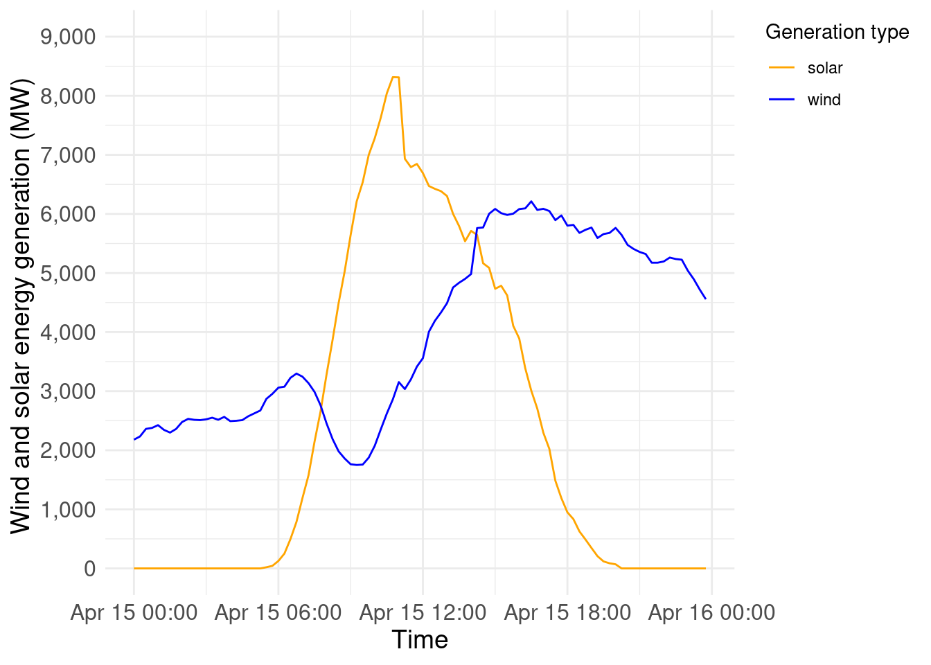
That’s all!